OpenVibe Designer :
OpenViBE is a software platform dedicated to designing, testing and using brain-computer interfaces. The package includes a Designer tool to create and run custom applications, along with several pre-configured and demo programs which are ready for use. To start with, go through the official documentation at http://openvibe.inria.fr/start/
Step1:
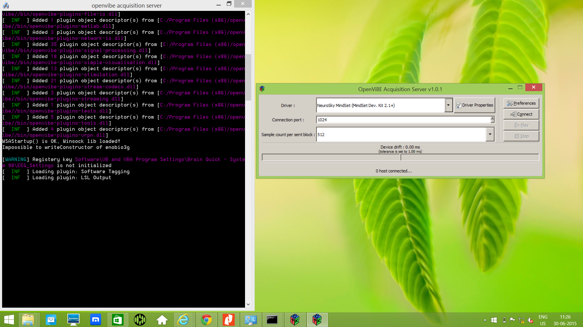
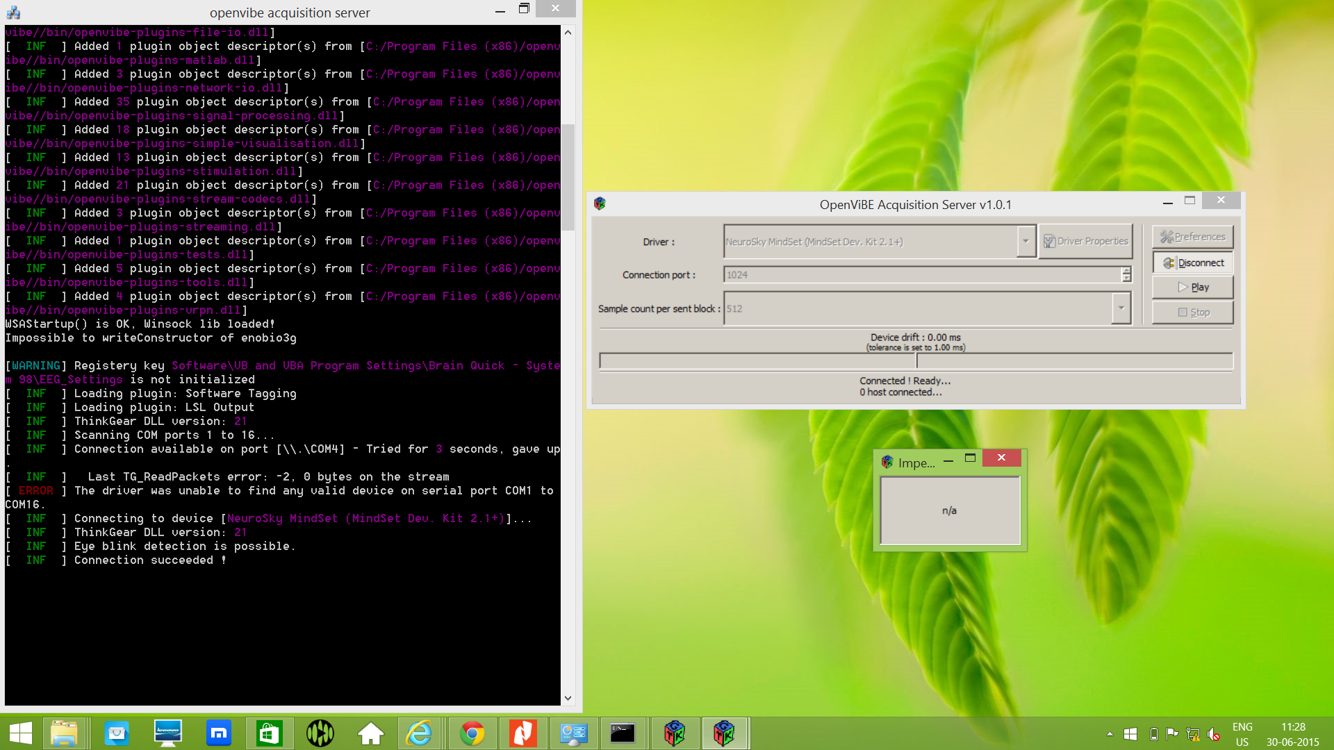
Open the OpenVibe Acquisition Server as shown below to setup and configure the neurosky headset.
Step2:
Select the driver as ‘ Neurosky Mindset (Mindset Dev Kit 2.1+) The device can be configured using ‘Driver Properties’ Preferably stick to the default connection port. Set the sample count sent per block to 512. Press ‘Connect’ and then ‘Play’ Acquisition server will now start Receiving data from the device and send it to the connected hosts
OpenVibe Designer
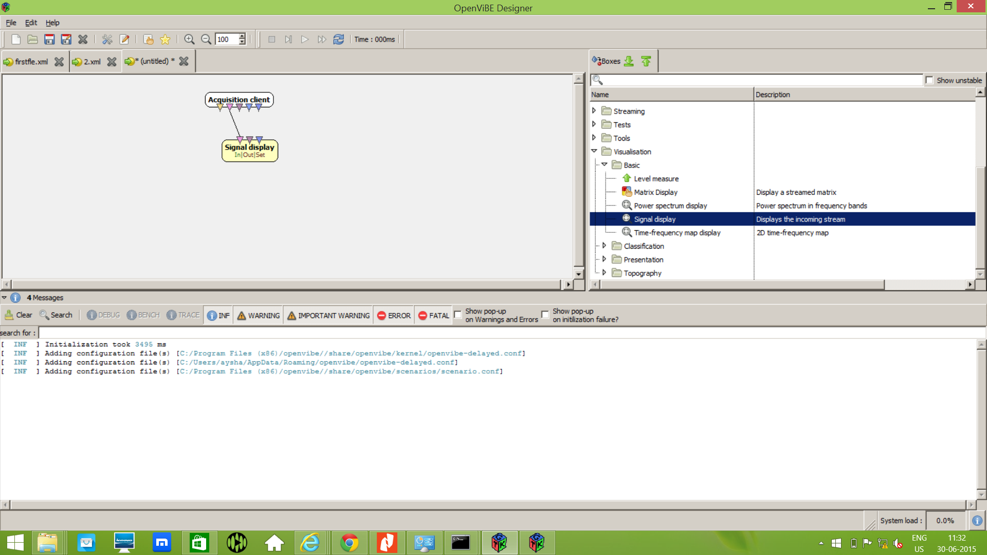
After configuring the port and device open the OpenVibe Designer. Let us display the signal acquired.
- Left click, drag and drop the box algorithm named ‘Acquisition Client’ to the workspace.
- Double click the same to configure it. This process is applicable to almost all the boxes. Also make sure that there is no discrepancy in the connection port value.
- In order to get a simple visualization of EEG, go to Visualization >> Basic Signal Display, and connect it to the ‘Acquisition Client’ box that you have already added.[Select one of the boxes, left click and connect the wire that appears in the second box.
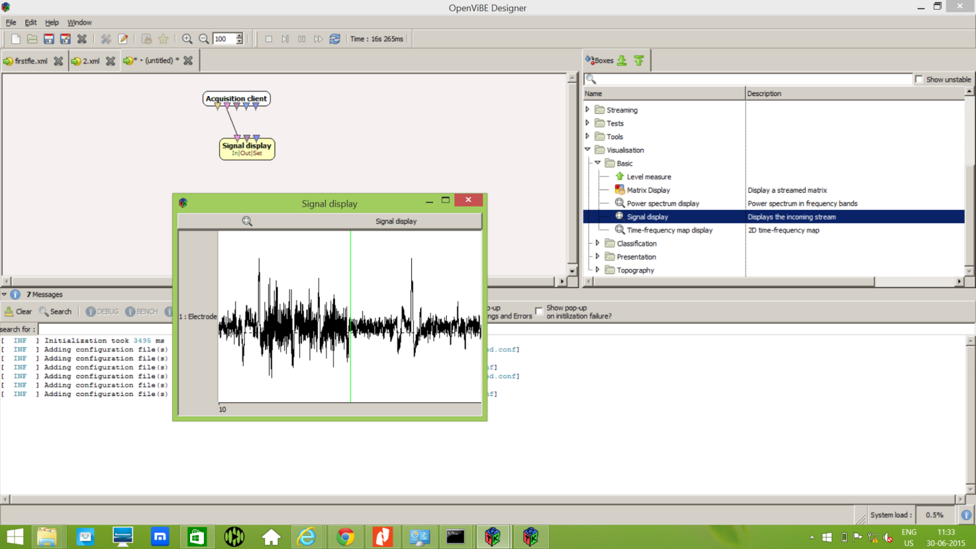
- As soon as we press Play button, the Signal Display Box opens as below
Working with Matlab
You can start with doing analysis with inbuilt toolboxes and functionalities of Matlab using any publically available EEG
datasets. Here I am using dataset of BCI competition IV from the link below:
http://www.bbci.de/competition/iv/#dataset2a
You can download the signals and unzip the files onto your default Matlab Folder. And load the 1st file onto the
workspace as below:
--> load('BCICIV_eval_ds1g.mat'); $ This will load the first file of the datasetGiven are continuous signals of 59 EEG channels and, for the calibration data, markers that indicate the time points of cue presentation and the corresponding target classes. Data are provided in Matlab format (*.mat) containing variable: cnt: the continuous EEG signals, size [time x channels]. The array is stored in datatype INT16. To convert it to uV values,
use cnt= 0.1*double(cnt); in Matlab.
To plot the first channel data type:
-->plot(cnt(:,1)) $ This will load the first file of the datasetGiven are continuous signals of 59 EEG channels and, for the calibration data, markers that indicate the time points of cue presentation and the corresponding target classes. Data are provided in Matlab format (*.mat) containing variable: cnt: the continuous EEG signals, size [time x channels]. The array is stored in datatype INT16. To convert it to uV values, use cnt= 0.1*double(cnt); in Matlab.
To plot the first channel data type:
---> plot(cnt(:,1))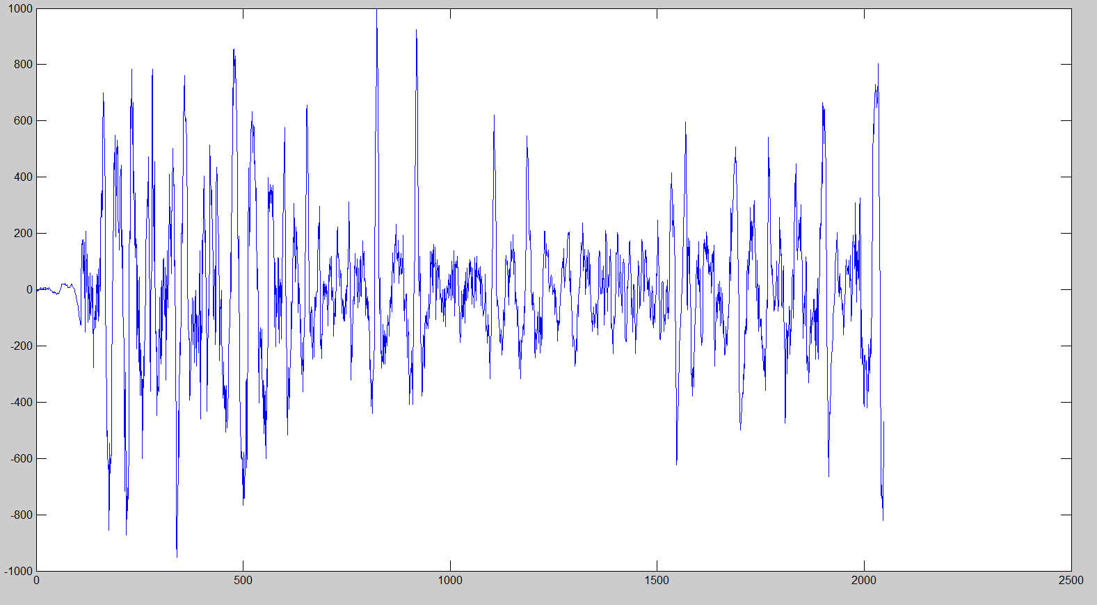
Taking a small Window of 2048 samples of 12 channels
--->A=cnt(1:2048,1:8);
---> fs=100;
---> ts=1/fs;
---> t=0:ts:2047*ts;
---> A=A';
---> A=double(A);
---> [no_of_channels, no_of_samples]=size(A);
---> plot(A(1,:))
Applying a High pass filter
---> Fstop = 1;    % Stopband Frequency
---> Fpass = 2;    % Passband Frequency
---> Astop = 60;   % Stopband Attenuation (dB)
---> Apass = 1;    % Passband Ripple (dB)
---> Fs    = 100;  % Sampling Frequency
---> h = fdesign.highpass('fst,fp,ast,ap', Fstop, Fpass, Astop, Apass, Fs);
---> Hd = design(h, 'equiripple', ...   'MinOrder', 'any', ...  'StopbandShape', 'flat');
---> filtered_data=filter(Hd,A,2);
Now plot the data
---> plot(filtered_data(:,1))
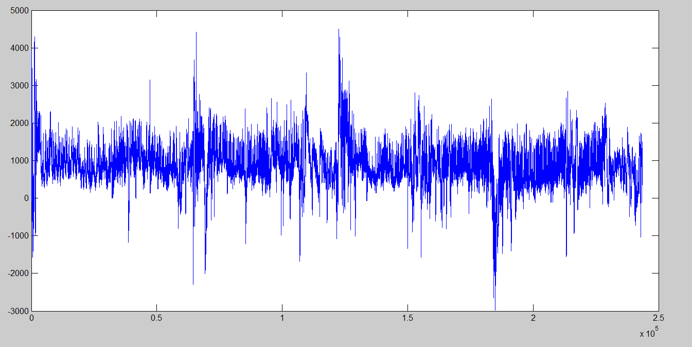
Calculating the Fast Fourier Transform
--> f=-fs/2:fs/no_of_samples:fs/2-fs/no_of_samples;
---> X=fft(double(A(1,:)),no_of_samples);
---> X=fftshift(X);
---> Xmag=abs(X);
---> Xphase=phase(X);
---> plot(f,Xmag)
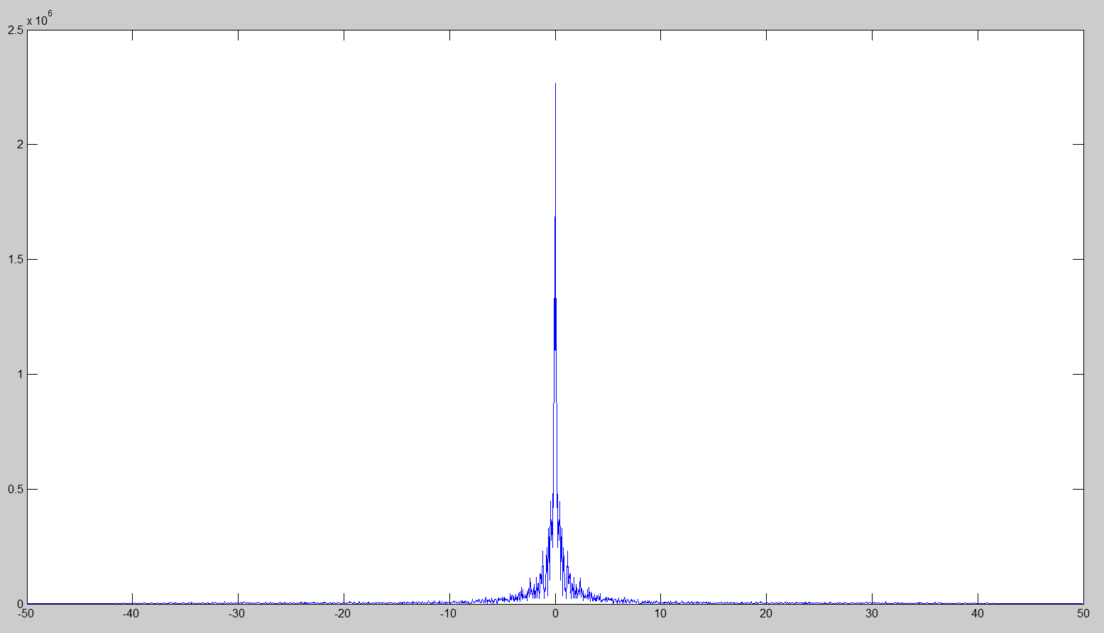
Before High-pass Filter
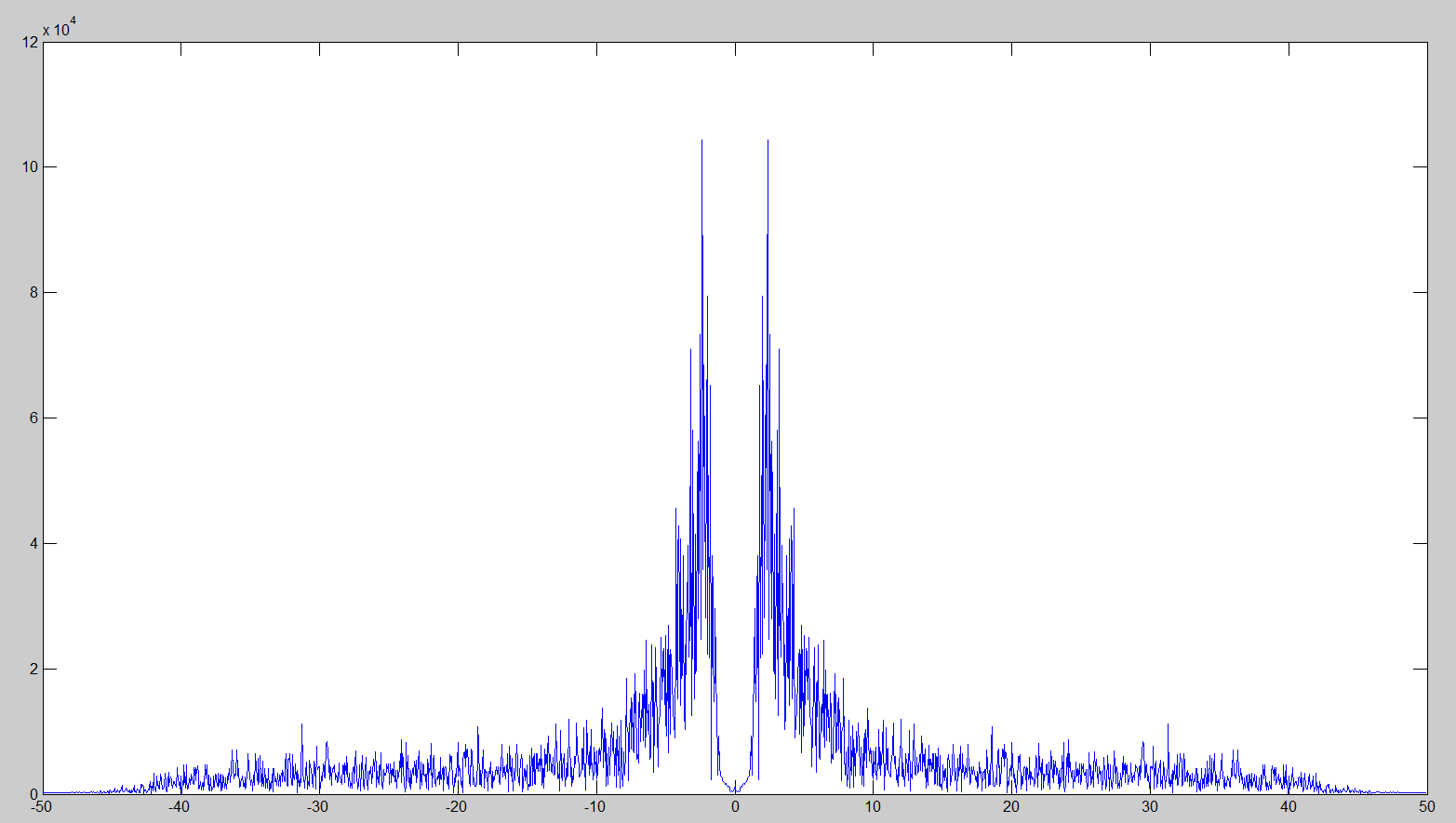
After High-pass Filter
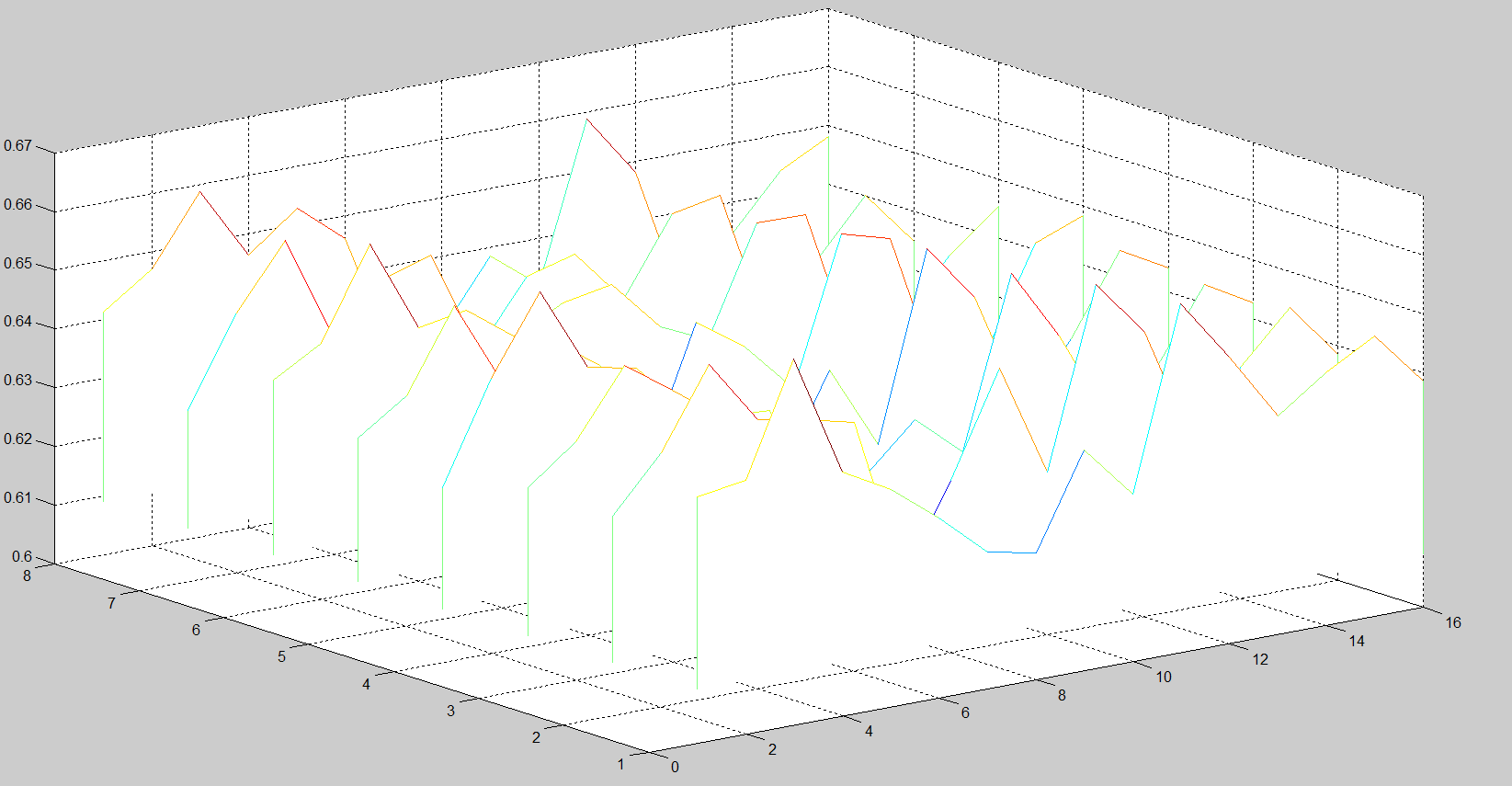
Finding The Shannon entropy
---> no_of_bins = 256;
---> windowsize = 128;
---> no_of_windows = round(no_of_samples/windowsize);
---> A=double(A);
---> probability = zeros(no_of_windows,no_of_bins);
---> entropy= zeros(1,no_of_windows);
for i=1:no_of_channels
for j = 1:no_of_windows
probability(j,:) = hist(A(i,((j-1)*windowsize+1):j*windowsize),no_of_bins)/no_of_samples;
entropy(i,j) = -sum(probability(j,:).*log2(0.0000000001+probability(j,:)));
end
end
Plot Entropyy
---> waterfall(entropy)