Once you run the files, a file can be saved in the MATLAB folder by using the Save option in the File menu in the Simulink window, or by hitting Ctrl-S in Simulink.
To open a previously saved file, use the Open option in the File menu in the Simulink window, or you could even do so by hitting Ctrl-O in Simulink.
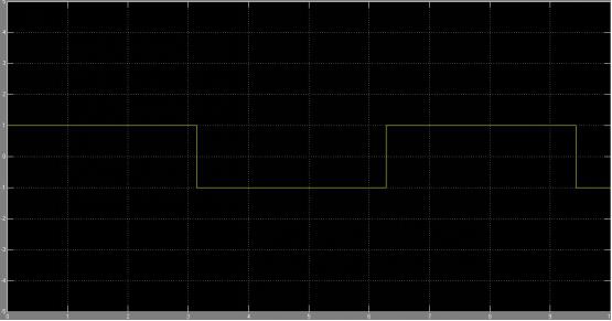
SOLUTIONS TO ASSIGNMENT 1
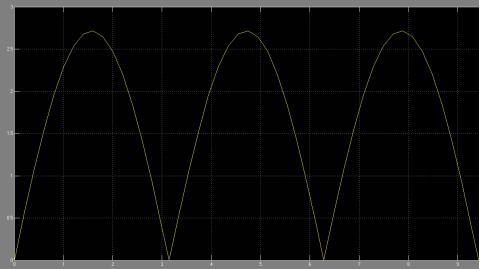
Output of which would be
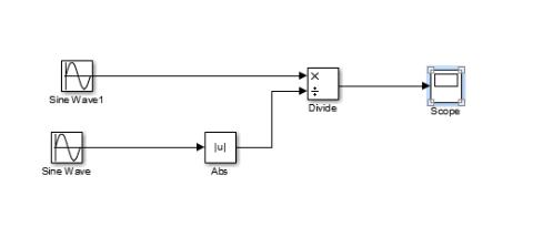
SOLUTIONS TO ASSIGNMENT 2

CONTROLS TUTORIALS FOR SIMULINK
The two main objects of use in Simulink are (1) Blocks & (2) Lines
Blocks are used to create, modify and display signals.
Lines are used to transmit signals from one block to another.
BLOCKS
Blocks can be of various types:
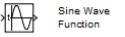
Sources:
Used in the generation of signals


Sinks:
Used to output or display signals


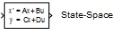
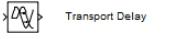
Continuous-time system elements

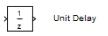
Discrete-linear time system elements


Math Operations: contains many common math operations


These blocks can have zero to any number of inputs or outputs. Unused terminals are shown as small open triangles.
LINES
The blocks are connected via lines which primarily define the direction of signal flow from the output of one block to the input of the next block. At time it may be necessary to split the signal into two to serve as an input to two blocks; there exist two ways to do this.
- First place the cursor at the point where it is needed to branch the line, then use the CTRL key in conjunction with the left mouse button and drag to the desired destination.
- Use the right mouse button and drag it to the desired destination.
MODELING OF A FIRST ORDER SYSTEM
To model any real time physical system in Simulink it is first necessary to create a mathematical model of the system. Thus we will take an example of the motion of a box on a floor with friction.
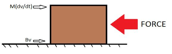
The horizontal forces can be represented in mathematical form as:
- V is considered as the instantaneous horizontal velocity(m/s) of the box
- Force(F) external horizontal force exerted on the box to propel it forward
- B is the damping coefficient (friction between the base of the box and floor)
- M is considered to be the mass of the block
On applying Newton’s Second law of motion we get
M*(dv/dt)=F-bv —- (1)
We thus consider our system constants as
M = 5 kg
B = 0.5 Nsm
On simplifying equation 1 we obtain
dv/dt= F-bv/M= (F-.5*v)/5 —(2)
Now that we have obtained a mathematical model of our system we can proceed to build the system model.
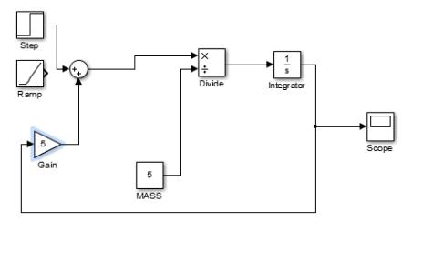
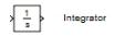
We would need a Sum block (F-bv); a divide block(1/M); an Integrator block(To integrate eq. 2)
(Refer the link on blocks to know where you could find these)
Next for proper utilisation of the blocks we need to edit these blocks. We can do so by double clicking on the block.
First for the sum block, since we need to subtract the damping force from the motor force we need to change the second sign. After double clicking the block; the sum block parameters window as in fig.Here we replace the ‘+’ in the list of signs text box with ‘–’
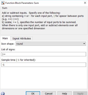
Sum parameters Window
Now that we have the functions setup we need connect them by a line originating from the output of sum block and input(x) of divide block.
It makes it easier to deal with Simulink if the functions and lines have appropriate tags.
To create a label fot the line, double click on the line and a cursor will appear.
For a function you can edit the already existing block by double clicking on its tag

Your workspace should look like this.
Now it is needed to use a constant block and edit its constant value to the mass (5) of the object.
Connect the constant blocks output to the second input of divide (÷).
Now connect the output of the divide function block to the integrator to obtain v from dv/dt
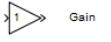
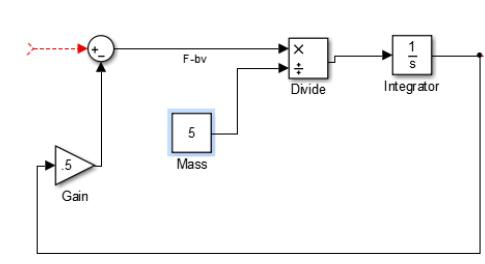
Since the damping force is a product of damping coefficient and velocity; we insert a gain block and edit the number gain value to b(.5) and connect the output of the integrator to the input of Gain.
The output of gain should be connected to the sum input block
Your system till now should appear as in below figure
In order to view the graphical output of the system a scope is used.
Connect the output of the Integrator to the input of the scope.
Input Force to the system
The force could be a (i)Step input or (ii)Ramp Input
Step input:
For Step input parameters involved are
Step time:
Time in seconds at which the step is desired
Initial Value:
Value of the signal before the step
Final Value:
Value of the signal after the step
Sample Time:
It is specified as a vector of two elements [Ts To]. Ts is the sampling time i.e. for a discrete model which produces its output every Ts seconds.
Ramp Input:
Ramp input parameters involved are
Slope:
rate at which the value is to rise per second
Start Time:
The value at which the ramp input is to begin
Initial output:
The initial value of the system before the ramp
Next add a scope to the system, which can be found under sinks in the Simulink library browser, and connect the output i.e. x to the input of the scope.